Example Run

Example Data and Running the Pipeline in Galaxy

Example read sets can be found here: https://share.corefacility.ca/index.php/s/BuX2EpLYbJbzmxB

These reads can then be uploaded into a galaxy instance and assembled into a collection.

See Running the workflow for how to run the pipeline in Galaxy.

Simple analysis of the Output in R

First download two datasets from the galaxy pipeline...

Blast results:

##: megablast REPLICON_DATABASE_NAME vs nucleotide BLAST database from data ##

SRST2 results:

##: Combine on data ##, data ##, and others

Depending on the number of samples and datasets in the history and the name of replicon database; the ## values and name will change.

For example...

Blast results:

88: megablast plasmidfinder_plusAMR.fasta vs nucleotide BLAST database from data 86

SRST2 results:

82: Combine on data 75, data 70, and others

In this next step we have renamed the files to srst2results.tsv and blastresults.tsv for simplicity and they reside in the R Project folder.

First attach the Plasmidprofiler package and then run it's main() function on the results:

library(Plasmidprofiler)  
main(blast.file = "blastresults.tsv", srst2.file = "srst2results.tsv")

This will run the following functions in order:

read_blast() - Import the blast file, add column names

blast_parser() - Parse imported file

amr_positives() - Detect AMR positive plasmids

read_srst2() - Import SRST2 file

combine_results() - Combine SRST2 and Blast

zetner_score() - Add Sureness value

amr_presence() - Add detected AMR to report

subsampler() - Apply filters to report

order_report() - Arrange report

save_files() - Save JPG and CSV

create_plotly() - Creates plot

save_files() - Save HTML plot

This will result in 3 files being created in the project directory all named P2Run.EXT where "EXT" is one of:

• png: for the static heat map
• html: for the interactive heat map
• csv: for the table of results

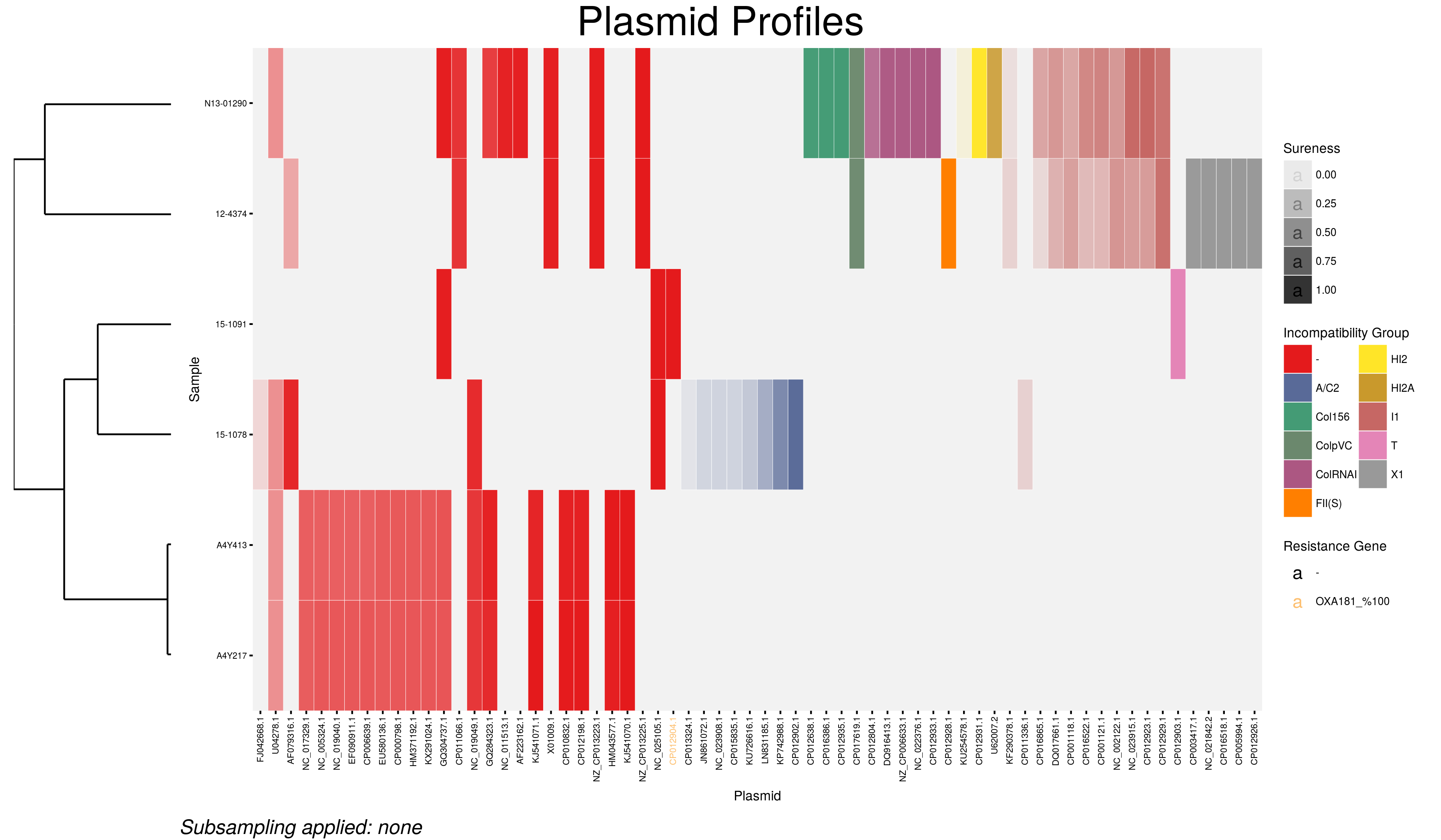
No filtering will have been done on these outputs because we did not specify any options in the function call. The static heat map therefore looks like this:

The options available to the main() function are:

blast.file - Either system location of blast results (tsv) or dataframe
srst2.file - Either system location of srst2 results (tsv) or dataframe
coverage.filter - Filters results below percent read coverage specified (eg. 80)
sureness.filter - Filters results below sureness specified (eg. 0.75)
length.filter - Filters plasmid sequences shorter than length specified (eg. 10000)
combine.inc - Flag to combine incompatibility sub-groups into their main type (set to 1)
plotly.user - Enter your plotly info to upload to Plotly
plotly.api - Enter your plotly info to upload to Plotly
post.plotly - Flag to post to Plotly
anonymize - Flag to anonymize plasmids and samples (set to 1)
main.title - A title for the figure

How about we change the title and restrict the plasmid results to thos >=4kb and with sureness of >=0.65?

main(blast.file = "blastresults.tsv", srst2.file = "srst2results.tsv", length.filter = 4000, sureness.filter = 0.65, main.title = "Restricted Dataset")

Now the heatmap looks more like this:

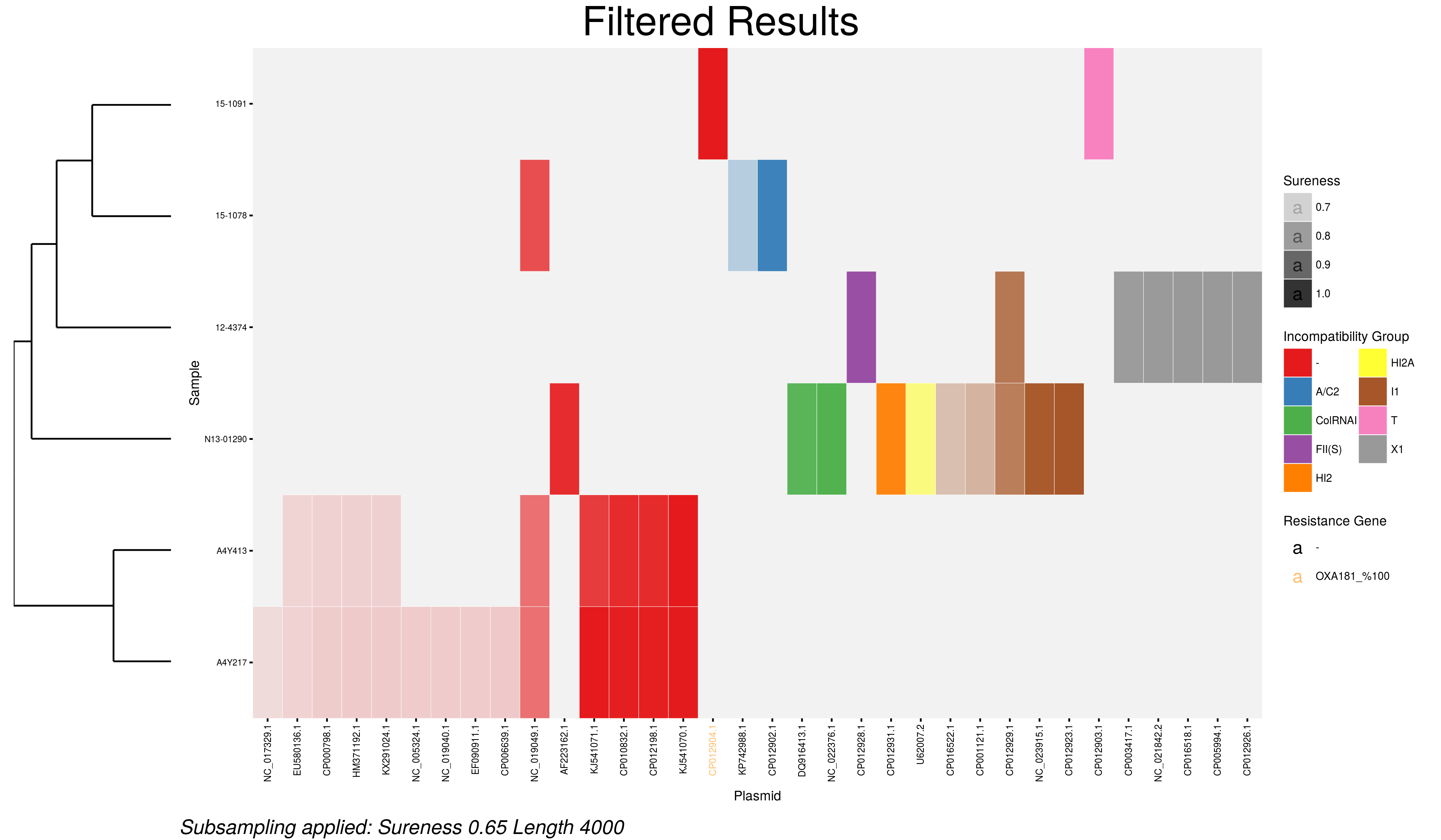
The corresponding interactive heat map and table of results will reflect these changes as well.

What do the results tell us?

The WGS reads from each sample have been analyzed and compared to the plasmid database from which the displayed plasmids were matched. The degree to which this match was made is displayed in the transparency of the individual plasmid cells of the heatmap according to the range of sureness chosen. Nearly transparent cells represent lower potential matches at the lowest end of the range and opaque cells near certainty that plasmid is represented in the sequencing data.

Each identified plasmid has been coloured and arranged according to its incompatibility group. The plasmids in which our genes of interest have been found are coloured according to the best gene hit found.

Examining the samples in order.

15-1091

• Two plasmids identified at high sureness.
• One belonging to the T incompatibility group (CP12903), the replicon of the other was not found in the Plasmid Finder database (CP12904)
• Plasmid CP12903 has been identified to carry the OXA181 gene of interest at 100% identity

15-1078

• Two different incompatibility groups identified, 3 total hits
• Examining the example table of results we can compare the two A/C2 hits and see that of the two, CP012902.1 is the better hit with 100% coverage and a lower sequence divergence.
• Because more than one plasmid of the same incompatibility group cannot persist in a cell at time we can conclude that the higher sureness hit is far more likely to be present than the other.

12-4374

• Three incompatibility groups identified: 3 plasmids likely to be present
• The plasmids from groups FII and I1 are easy to distinguish but what of the X1s? Each of them has a very high sureness score close to 1 (as seen in the example table of results) with near total coverage and very low sequence divergence. Plasmid CP012926.1 has the highest total sureness value at 0.999 and is therefore the most similar to the actual plasmid present.
• Again, only a single plasmid per incompatibility group is possible so although there are multiple high value hits, the best is more likely to be the present plasmid.

N13-01290

• A similar situation as above. Multiple plasmids from the incompatibility groups Col, HI2, HI2A, and I1 were found.
• A call must be made based on the sureness values which plasmid to consider present from each group. Of the two Col plasmids NC_022376 has higher sureness which translates to higher coverage and lower divergence and is the appropriate choice.
• The best hit plasmid from each of the groups are considered present.

A4Y217 and A4Y413

• No hits to plasmids with known incompatibility groups
• Each with a number of plasmids lacking known replicons in similar pattern
• In this case it is necessary to examine the best hits by researching their accession numbers to make a determination on which will be considered present.

Using the other package functions

There are a number of other package functions available to the user for data manipulation in R. To access them first attach the Plasmidprofiler package and import the output files of the pipeline into your R environment:

library(Plasmidprofiler)  
br <- read_blast("blastresults.tsv")  
sr <- read_srst2("srst2results.tsv")

Next perform the initial parsing and combine the data into the combined report:

br.parsed <- blast_parser(br)
pos.samples <- amr_positives(br)
cr <- combine_results(sr, br.parsed)

This results in a table with the following columns:

• Sample
• Plasmid
• Inc_group
• Coverage
• Divergence
• Length
• Clusterid

Next the sureness values must be calculated and the identified AMR genes / Genes of Interest added to the table:

cr <- zetner_score(cr)
cr <- amr_presence(cr, pos.samples)

If you wish to apply subsampling to the report subsampler() is the function for you. The available filters are as follows:

• Coverage: Filters results below percent read coverage specified
  eg. 95.9 cuts results where reads covered less than 95.9% of the total length

• Sureness: Filters results below sureness specified
  eg. 0.9 cuts results where the sureness falls below 0.9

• Length: Filters plasmid sequences shorter than length specified
  eg. 10000 cuts out results where the plasmid was less than 10kb

• Incompatibility groups can also be combined (eg. Fii(S) and Fii(K) are combined into Fii)

After applying filters (or not) the report must be ordered using order_report(). Changing to anonymize flag to 1 will result in sample and plasmid names being masked:

cr.filtered <- subsampler(cr, sure.filter = 0.85)
cr.ordered <- order_report(cr.filtered, anonymize = NA)

From this point data modification can be done. For example, concatenating sequence types to sample names:

metadata <- read.xlsx("Heatmap_metadata.xlsx", 1)

for(i in 1:length(cr.ordered$Sample)){
  ii <- match(cr.ordered[i, "Sample"], metadata[,1])
  if(is.na(ii)){
    print(paste(cr.ordered[i,"Sample"], "not found"))
    cr.ordered[i, "Sample2"] <- cr.ordered[i,"Sample"]
    next
  }
  cr.ordered[i, "Sample2"] <- paste(cr.ordered$Sample[i], '_', metadata[ii, "Organism"], '_', metadata[ii, "ST"], sep = '', collapees = '')
}

cr.ordered["Sample"] <- cr.ordered["Sample2"]
cr.ordered["Sample2"] <- NULL

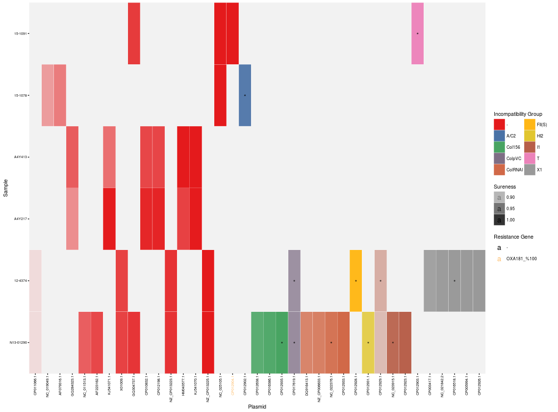
The heatmap alone can be plotted using the plot_heatmap() function. If desired, the longest plasmid of each incompatibility group can be highlighted. An interactive heatmap can be built using the create_plotly() function. The function create_grob() will assemble all the appropriate graphical objects into the full static heatmap:

plot_heatmap(cr.ordered, len.highlight = 1)
create_plotly(report, title = "Plasmid Profiles")
create_grob(cr.ordered)

Use the save_files() function to save the various outputs one at a time:

save_files(cr.ordered, plot.png = 1, report.csv = 1, webpage = NA)